But you may have a cell to which you have previously applied a fill color, only to find that the data has changed, or that the formatting of the document dictates the removal of that existing fill color. Fortunately, you are able to remove the existing fill color in Google Sheets and revert the cell to its default, fill color-less state. So continue reading our tutorial below and learn how to remove cell shading in Google Sheets.
How to Remove Cell Shading in Google Sheets
Our guide continues below with additional information on how to clear a cell’s fill color in Google Sheets, including pictures of these steps. If some of the text in your cells isn’t visible because it doesn’t fit within the boundaries of the cell, then our how to wrap text in Google Sheets article can show you how to fix it.
How to Remove the Background Fill Color from a Cell in Google Sheets (Guide with Pictures)
The steps in this article were performed in Google Chrome, in the Web browser version of Google Sheets. These steps assume that you currently have a cell with a fill color that you would like to remove. Note that we will be focusing primarily on removing an existing fill color with this article, but you can use very similar steps if you would like to change the fill color instead.
Step 1: Go to your Google Drive at https://drive.google.com/drive/my-drive and open the spreadsheet containing the fill color that you want to remove.
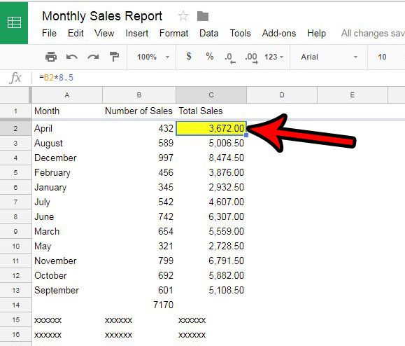
Step 2: Select the cell with the fill color to remove.
Note that you can hold down the Ctrl key and click multiple cells, if you would like to remove the fill color from more than one.
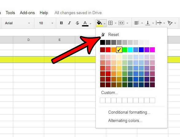
Step 3: Click the Fill color button in the toolbar above the spreadsheet, then click the Reset option.
Now that you know how to remove fill color in Google Sheets you will be able to use this technique when you want to get rid of an existing fill or background color in your cells, or if you want to add color to some of your cells instead. Do you need to add a column to the middle of your spreadsheet and you’re worried about cutting and pasting everything to make room for the new column? Learn a simple way to insert columns in Google Sheets that simply moves your existing columns over.
How to Add Yellow Shading to a Row in Google Sheets
Large spreadsheets can be much easier to manage when you use fill colors to highlight rows that are important, or share similarities. For example, highlighting multiple rows with a yellow fill color could let you highlight good months in a sales report. It draws the attention of the reader without affecting the data in the spreadsheet. But if you want to highlight your cells with fill color, you might not be sure how to do so. Our article below will show you how to select a row in Google Sheets and apply a fill color to that row. If you need to combine some of the cells in that row into one big cell, then learn how to use the cell merging feature in Google Sheets to achieve that result.
How to Use Fill Color in Google Sheets
The steps in this article were performed in the Google Sheets application that is accessible through the Google Chrome Web browser. Once you complete the steps in this guide, you will have a row (or rows) in your Google Sheets spreadsheet that have a fill color that you select. You can use this same method to apply a fill color to a column, or to a group of cells.
Step 1: Sign into your Google Drive at https://drive.google.com/drive/my-drive and open the spreadsheet to which you wish to add fill color to a row or rows.
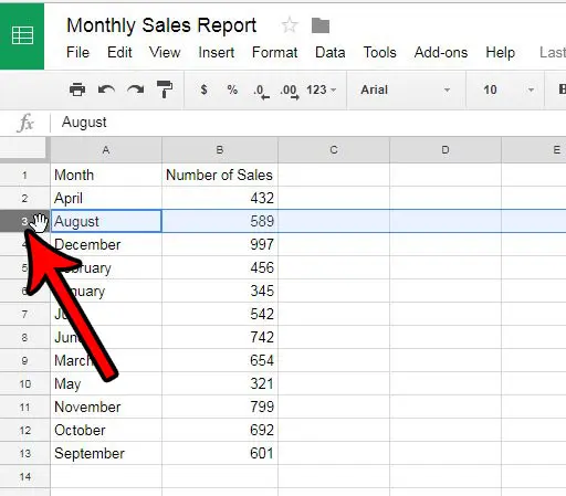
Step 2: Click the row number to the left of the spreadsheet to select the entire row.
Note that you can select multiple rows by holding down the Ctrl key on your keyboard and clicking additional rows.
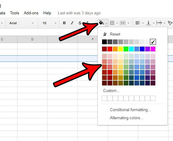
Step 3: Click the Fill Color button in the toolbar at the top of the window, then select the color that you want to use to fill the selected row.
If you wish to remove the fill color from a selected row, then click the Reset button at the top of the Fill Color menu from step 3. When you expand the Fill color drop down menu, note that there are options at the bottom for Conditional formatting and Alternating colors. You can use conditional formatting if you would like to have Google Sheets change the fill color automatically based on a set of criteria. You can use the Alternating colors option if you want to have a pattern of colors for your cell fill colors. Do you have a spreadsheet on which you need to change the width of a lot of columns? Learn how to change multiple column widths in Google Sheets so that you don’t need to change each column individually.
Additional Sources
After receiving his Bachelor’s and Master’s degrees in Computer Science he spent several years working in IT management for small businesses. However, he now works full time writing content online and creating websites. His main writing topics include iPhones, Microsoft Office, Google Apps, Android, and Photoshop, but he has also written about many other tech topics as well. Read his full bio here.
You may opt out at any time. Read our Privacy Policy


